Introduction

This page is the continuation of my blog post on R commands. On the blog, see also why use R and the RSS feed of posts labelled R.

History of R

Exploratory data analysis

“Tukey defined data analysis in 1961 as:”Procedures for analyzing data, techniques for interpreting the results of such procedures, ways of planning the gathering of data to make its analysis easier, more precise or more accurate, and all the machinery and results of (mathematical) statistics which apply to analyzing data. Tukey’s championing of EDA encouraged the development of statistical computing packages, especially S at Bell Labs. The S programming language inspired the systems S-PLUS and R. This family of statistical-computing environments featured vastly improved dynamic visualization capabilities, which allowed statisticians to identify outliers, trends and patterns in data that merited further study.”

S programming language

“S is one of several statistical computing languages that were designed at Bell Laboratories, and first took form between 1975–1976. Up to that time, much of the statistical computing was done by directly calling Fortran subroutines; however, S was designed to offer an alternate and more interactive approach, motivated in part by exploratory data analysis advocated by John Tukey. Early design decisions that hold even today include interactive graphics devices (printers and character terminals at the time), and providing easily accessible documentation for the functions.”

See also the comparison between R and Python below.

Control flow

dplyr::case_when is a generalised vectorised if. Example use:

 x <- 1:50
 case_when(
   x %% 35 == 0 ~ "fizz buzz",
   x %% 5 == 0 ~ "fizz",
   x %% 7 == 0 ~ "buzz",
   TRUE ~ as.character(x)
 )

Data table

Database like operation benchmark between data table, dplyr, python pandas and other database like tools.

Data types

Data frames

The data type used in must analysis. Data frames are an aligned collection of vectors with observation in rows and variables in columns.

Size in memory

Print the size of a data frame in memory

print(object.size(df), units="MB")

Vectors

Everything is a vector

There are no scalar values in R, only vectors, this makes it very natural to process times series or cross sectional data over many N observations as if we were processing only one instance of the variable.

SO answer concerning indexing up to end of vector/matrix “Sometimes it’s easier to tell R what you don’t want”

x <- c(5,5,4,3,2,1)
x[-(1:3)]
x[-c(1,3,6)]

Set operations

x = letters[1:3]
y = letters[3:5]
union(x, y)

## [1] "a" "b" "c" "d" "e"

intersect(x, y)

## [1] "c"

setdiff(x, y)

## [1] "a" "b"

setdiff(y, x)

## [1] "d" "e"

setequal(x, y)

## [1] FALSE

Dates

Create a date vector

as.Date("2022-01-01")
seq(as.Date("2022-01-01"), by=1, len=3)

Parse a character vector into a date vector with lubridate

tralala_chr <- c("202012", "202101")
tralala <- lubridate::parse_date_time(tralala_chr, "%y%m")
tralala

Represent the date object as a string

format(min(tralala),"%Y-%m")
format(max(tralala),"%Y-%m")

Factors

My answer to the question how to reorder factor levels the tidy way

If you happen to have a character vector to order, for example:

iris2 <- iris %>%
    mutate(Species = as.character(Species)) %>%
    group_by(Species) %>%
    mutate(mean_sepal_width = mean(Sepal.Width)) %>%
    ungroup()

You can also order the factor level using the behavior of the forcats::as_factor function :

"Compared to base R, this function creates levels in the order in which they appear"

library(forcats)
iris2 %>%
    # Change the order
    arrange(mean_sepal_width) %>%
    # Create factor levels in the order in which they appear
    mutate(Species = forcats::as_factor(Species)) %>%
    ggplot() +
    aes(Species, Sepal.Width, color = Species) +
    geom_point()

Notice how the species names on the x axis are not ordered alphabetically but by increasing value of their mean_sepal_width. Remove the line containing as_factor to see the difference.

Strings

message("Using the following letters: ", paste(letters, collapse=","), ".")

## Using the following letters: a,b,c,d,e,f,g,h,i,j,k,l,m,n,o,p,q,r,s,t,u,v,w,x,y,z.

stringsAsFactors: An unauthorized biography

“The argument ‘stringsAsFactors’ is an argument to the ‘data.frame()’ function in R. It is a logical that indicates whether strings in a data frame should be treated as factor variables or as just plain strings. […] By default, ‘stringsAsFactors’ is set to TRUE.” “Most people I talk to today who use R are completely befuddled by the fact that ‘stringsAsFactors’ is set to TRUE by default. […]” “In the old days, when R was primarily being used by statisticians and statistical types, this setting strings to be factors made total sense. In most tabular data, if there were a column of the table that was non-numeric, it almost certainly encoded a categorical variable. Think sex (male/female), country (U.S./other), region (east/west), etc. In R, categorical variables are represented by ‘factor’ vectors and so character columns got converted factor. […] Why do we need factor variables to begin with? Because of modeling functions like ‘lm()’ and ‘glm()’. Modeling functions need to treat expand categorical variables into individual dummy variables, so that a categorical variable with 5 levels will be expanded into 4 different columns in your modeling matrix.” […]

“Around June of 2007, R introduced hashing of CHARSXP elements in the underlying C code thanks to Seth Falcon. What this meant was that effectively, character strings were hashed to an integer representation and stored in a global table in R. Anytime a given string was needed in R, it could be referenced by its underlying integer. This effectively put in place, globally, the factor encoding behavior of strings from before. Once this was implemented, there was little to be gained from an efficiency standpoint by encoding character variables as factor. Of course, you still needed to use ‘factors’ for the modeling functions.”

Levenshtein distance between words

Cf. https://en.wikipedia.org/wiki/Levenshtein_distance and help(adist).

adist("kitten", "sitting")

##      [,1]
## [1,]    3

Capitalise first letter

Capitalise the first letter of each word

stringr::str_to_title("bla bla bla")
# [1] "Bla Bla Bla"

Lists

Given a list structure x, unlist simplifies it to produce a vector which contains all the atomic components which occur in x.

l1 <- list(a="a", b="2,", c="pi+2i")
str(l1)

## List of 3
##  $ a: chr "a"
##  $ b: chr "2,"
##  $ c: chr "pi+2i"

unlist(l1) # a character vector

##       a       b       c 
##     "a"    "2," "pi+2i"

str(unlist(l1))

##  Named chr [1:3] "a" "2," "pi+2i"
##  - attr(*, "names")= chr [1:3] "a" "b" "c"

Extract the first element of a nested list SO

minyearmaxyear <- list(c(2001, 2009), c(2010, 2014), c(2015, 2100))
library(purrr)
map(minyearmaxyear, 1)

## [[1]]
## [1] 2001
## 
## [[2]]
## [1] 2010
## 
## [[3]]
## [1] 2015

Remove items from a list

Remove elements from a named list in R.

l <- list(a = 1, b = 2)
l <- within(l, rm(a))

Remove elements from an unnamed list

l <- list(1,2)
l[1] <- NULL

Bind data frames in a list

# Large list if data frames
l_df <- list(head(iris), iris[c(92:95),], tail(iris))
df_stack <- data.frame()
for (i in 1:length(l_df)){
    # Bind the first list item and remove it
    df_stack <- rbind(df_stack, l_df[[1]])
    l_df[1] <- NULL
}
# Reset row names
row.names(df_stack) <- NULL

This will take less memory than binding the data frame in this way:

l_df <- list(head(iris), iris[c(92:95),], tail(iris))
dfdt = data.table::rbindlist(l_df)

And should give a similar result

identical(df_stack, data.frame(dfdt))
# TRUE

S3 methods

List all available methods for a class:

methods(class="lm")

Debug

Hadley Wickham on debugging

“NB: You shouldn’t need to use these tools when writing new functions. If you find yourself using them frequently with new code, reconsider your approach. Instead of trying to write one big function all at once, work interactively on small pieces. If you start small, you can quickly identify why something doesn’t work, and don’t need sophisticated debugging tools.”

Debug with base R

Print the call stack of the last error:

traceback()

Start a browser at a particular position in code:

 browser()

Next, n: executes the next step in the function. If you have a variable named n, you’ll need print(n) to display its value.

Step into, or s: works like next, but if the next step is a function, it will step into that function so you can explore it interactively.

Finish, or f: finishes execution of the current loop or function.

Continue, c: leaves interactive debugging and continues regular execution of the function. This is useful if you’ve fixed the bad state and want to check that the function proceeds correctly.

Stop, Q: stops debugging, terminates the function, and returns to the global workspace. Use this once you’ve figured out where the problem is, and you’re ready to fix it and reload the code.

Debug with rlang

Print the call stack of the last error in simplified form:

rlang::last_error()

Print the full call stack of the last error:

rlang::last_trace()

More information on the behaviour of backtrace:

help(trace_back, package=rlang)

“Because of lazy evaluation, the call stack in R is actually a tree, which the ‘summary()’ method of this object will reveal.”

Environnement

R environment

List objects in the global environment:

ls

List objects coming from a specific loaded package:

ls("package:stats")
ls("package:stats", pattern="smooth")

Remove all objects in the environment except one:

rm(list=ls()[!ls()=="object_to_keep"]) 
rm(list=ls()[!ls()=="con"]) # Remove all except a database connection

Get the current environment

rlang::current_env()

Read system environment variables

Read an environment variable from the operating system

data_path <- Sys.getenv("PROJECT_DATA")

Editors

I use Vim and the great Nvim-R plugin to edit R markdown documents and R scripts. I browse the table of content of R markdown files with the Voom plugin. I create R packages with Makefiles. I use the fugitive plugin to manage my git commits. See my Vim page for more information.

Rstudio is a great editors for those who prefer a graphical user interface. It has a Vim mode. In fact I trained my muscle memory for Vim movement keys inside RStudio initially. Rstudio also has a lot of menus and buttons to work with Rmarkdown documents, view the state of a git repository and build packages.

Input output

getwd()
list.files(tempdir()) 
dir.create("blabla")

Apache Arrow and parquet files

Apache arrow R packages

“Read and write Feather files (read_feather(), write_feather()), a format optimized for speed and interoperability”

library(arrow)
read_parquet() # to read a single file
open_dataset() # to open a dataset sharded over multiple files

help(open_dataset)

” Call ‘open_dataset()’ to point to a directory of data files and return a ‘Dataset’, then use ‘dplyr’ methods to query it.”’

library(arrow)
library(dplyr)
# Set up directory for examples
tf <- tempfile()
dir.create(tf)
on.exit(unlink(tf))

data <- dplyr::group_by(iris, Species)
write_dataset(data, tf)

# open only the setosa part
setosa <- open_dataset(tf) %>%
    filter(Species == "setosa") %>%
    collect()

CSV files

Read one csv file with default R function.

read.csv("data.csv", )

Read many csv files with functions from the tidyverse packages.

First write sample csv files to a temporary directory. It’s more complicated than I thought it would be.

library(dplyr)
library(purrr)
library(purrrlyr)
library(readr)
data_folder <- file.path(tempdir(), "iris")
dir.create(data_folder)
iris %>%
    # Keep the Species column in the output
    # Create a new column that will be used as the grouping variable
    mutate(species_group = Species) %>% 
    group_by(species_group) %>%
    nest() %>%
    by_row(~write.csv(.$data, 
                      file = file.path(data_folder, paste0(.$species_group, ".csv")),
                      row.names = FALSE))

Read these csv files into one data frame. Note the Species column has to be present in the csv files, otherwise we would loose that information.

iris_csv <- list.files(data_folder, full.names = TRUE) %>% 
    map_dfr(read_csv)

write_csv returned an Error in write_delim(...) is.data.frame(x) is not TRUE That’s why we used write.csv instead.

RDS files

RDS is a Serialization Interface for Single Objects. Objects are saved to binary data and compressed to the gzip format, see help(saveRDS) for more details.

Write a dataset to an rds file:

saveRDS(iris, "/tmp/iris.rds")

Read a dataset from an rds file

iris2 <- readRDS("/tmp/iris.rds")
identical(iris, iris2)

Databases

Dplyr has databases backends to MySQl (MariaDB) and PostgreSQL.

Create directories

Create a directory do not show a warning if it exists already.

dir_path = "/tmp/blabla/"
dir.create(dir_path, showWarnings = FALSE)

Find and replace

Longest contiguous stretch of non-NAs:

na.contiguous(c(NA,1:3,NA,NA,3:5,NA,NA))
] 1 2 3
tr(,"na.action")
]  1  5  6  7  8  9 10 11
tr(,"class")
] "omit"
tr(,"tsp")
] 2 4 1
na.contiguous(c(NA,1:3,NA,NA,3:6,NA,NA))
] 3 4 5 6
tr(,"na.action")
]  1  2  3  4  5  6 11 12
tr(,"class")
] "omit"
tr(,"tsp")
]  7 10  1

Replace text in column names

Add the first row to the column name, useful for some double headed csv files coming from pandas.

paste(names(df), df[1,])

Replace a regular expression with optional numerical pattern and final space

names(df) <- gsub(".per.hectare.[0-9]* *", "_", names(df))

Using and, or in a regular expression

Change columns to snake case

column_names <- c("Bla, Bla", "Hips, Hops", "Yield/Carcass Weight",
                  "Production", "Producing Animals/Slaughtered",
                  "Area harvested", "Yield")
gsub("[^[:alnum:]]","_",tolower(column_names))

## [1] "bla__bla"                      "hips__hops"                   
## [3] "yield_carcass_weight"          "production"                   
## [5] "producing_animals_slaughtered" "area_harvested"               
## [7] "yield"

# Replace one or more occurrences by an underscore
gsub("[^[:alnum:]]+","_",tolower(column_names))

## [1] "bla_bla"                       "hips_hops"                    
## [3] "yield_carcass_weight"          "production"                   
## [5] "producing_animals_slaughtered" "area_harvested"               
## [7] "yield"

iris2 <- iris
names(iris2) <- gsub("[^[:alnum:]]+","_",tolower(names(iris2)))
print(names(iris))

## [1] "Sepal.Length" "Sepal.Width"  "Petal.Length" "Petal.Width"  "Species"

# [1] "sepal_length" "sepal_width"  "petal_length" "petal_width"  "species"

Installing R and packages

To install R and Rstudio on Debian, see the debian.html#r_and_rstudio page on this site.

To install packages simply enter the following at an R command prompt:

install.packages("package_name")

Some packages have dependencies that need to be installed at the OS level. Error messages:

"Configuration failed because libcurl was not found." 
"Configuration failed because libxml-2.0 was not found."
"Configuration failed because openssl was not found."

Can be solved by installing these dependencies:

sudo apt install libcurl4-openssl-dev 
sudo apt install libxml2-dev 
sudo apt install libssl-dev

Install from source file

To install from a source file

install.packages("~/rp/FAOSTATpackage/FAOSTAT_2.2.1.tar.gz", repos=NULL)

System information used by install.packages() to determine default installation parameters

getOption("repos")
getOption("pkgType")

Eurostat Package

Install required GDAL development library for the “sf” package

sudo apt install libgdal-dev

Then at the R prompt

install.packages("eurostat")

Information about your R system

sessionInfo()
installed.packages()

R Markdown

Create websites

Rmarkdown site generator

This website is generated from R Markdown documents with:

 Rscript -e "rmarkdown::render_site()"

The advantage of the rmarkdown site generator is that it creates pages with a floating, foldable table of content. It’s nice for pages that have a lot of subdivisions like this blog. The structure of a website is specified in a yaml file. For example, the code below creates a navigation bar:

navbar:
  title: "Paul Rougieux"
  left:
    - text: "Home"
      icon: fa-home 
      href: index.html
    - text: "Tools"
      icon: fa-wrench
      menu:
        - text: "Bash"
          href: bash.html

Bookdown site generator

For blogs that fit into a book structure, with chapters, the bookdown package create a single clickable table of content for the whole site. It can also export the content to pdf format.

Specifying input from many sub directories in _bookdown.yml:

rmd_files: ["index.Rmd", "chapters/chapt1.RMD", "chapters/chapt2.RMD"]

Attention this will only work in the Merge and Knit strategy, as explained in the book chapter on two rendering approaches

“We call these two approaches “Merge and Knit” (M-K) and “Knit and Merge” (K-M), respectively.” “K-M does not allow Rmd files to be in subdirectories, but M-K does.”

Cross references

R markdown cross ref

“Cross-referencing is not provided directly within the base rmarkdown package, but is provided as an extension in bookdown (Xie 2020c). We must therefore use an output format from bookdown (e.g., html_document2, pdf_document2, and word_document2, etc.) in the YAML output field.”

Bookdown issue with flextable Table and figure cross references in word Now solved with the following implementation

iris %>% head() %>% flextable()

This is a reference to flextable @ref(tab:irishead). The chunk name should not contain an underscore, otherwise the cross reference will not work. See bookdown issue 941.

See more flextable caption examples in system.file(package = "flextable", "examples", "rmd", "captions")

Flextable and officer package

The officer package makes it possible to create improved word and powerpoint documents. The flextable package has a few functions to generate tables for word documents (otherwise they look funny).

Before installing flextable, the following system dependencies were required:

sudo apt install libcairo2-dev libjpeg-dev libgif-dev

Installation in R:

install.packages("flextable")

This is to work with colleagues who are not in the latex/pdf world.

Landscape pages

library(officer)
library(flextable)
ft_iris <- iris %>%
    head() %>%
    flextable() %>%
    autofit()
# Add a flex table in landscape format 
# Supply document name here, otherwise start an empty doc
doc <- read_docx() %>% 
  # Portait and landscape sections are defined by their ending
  # A portrait section is ending here
  body_end_section_portrait() %>%
  body_add_flextable(value = ft_iris, split = TRUE) %>%
  # A landscape section is ending here
  body_end_section_landscape() %>% 
  print(target = "/tmp/iris.docx")

kable to create tables

A table caption

knitr::kable(head(iris), caption = "An example table caption.")

An example table caption.
Sepal.Length	Sepal.Width	Petal.Length	Petal.Width	Species
5.1	3.5	1.4	0.2	setosa
4.9	3.0	1.4	0.2	setosa
4.7	3.2	1.3	0.2	setosa
4.6	3.1	1.5	0.2	setosa
5.0	3.6	1.4	0.2	setosa
5.4	3.9	1.7	0.4	setosa

Examples copie from yihui’s R markdown cookbook.

set.seed(100)
d <- cbind(X1 = runif(3), 
           X2 = 10^c(3, 5, 7), 
           X3 = rnorm(3, 0, 1000))
# at most 4 decimal places
knitr::kable(d, digits = 4)

X1	X2	X3
0.3078	1e+03	-1585.8810
0.2577	1e+05	-40.6920
0.5523	1e+07	-331.0045

# round columns separately
knitr::kable(d, digits = c(5, 0, 2))

X1	X2	X3
0.30777	1e+03	-1585.88
0.25767	1e+05	-40.69
0.55232	1e+07	-331.00

# do not use the scientific notation
knitr::kable(d, digits = 3, format.args = list(scientific = FALSE))

X1	X2	X3
0.308	1000	-1585.881
0.258	100000	-40.692
0.552	10000000	-331.005

# add commas to big numbers
knitr::kable(d, digits = 3, format.args = list(big.mark = ",",
  scientific = FALSE))

X1	X2	X3
0.308	1,000	-1,585.881
0.258	100,000	-40.692
0.552	10,000,000	-331.005

The format is recognised automatically by knitr based on the nature of the output document.

cat(kable(head(iris, 1), format = "html"))

## <table>
##  <thead>
##   <tr>
##    <th style="text-align:right;"> Sepal.Length </th>
##    <th style="text-align:right;"> Sepal.Width </th>
##    <th style="text-align:right;"> Petal.Length </th>
##    <th style="text-align:right;"> Petal.Width </th>
##    <th style="text-align:left;"> Species </th>
##   </tr>
##  </thead>
## <tbody>
##   <tr>
##    <td style="text-align:right;"> 5.1 </td>
##    <td style="text-align:right;"> 3.5 </td>
##    <td style="text-align:right;"> 1.4 </td>
##    <td style="text-align:right;"> 0.2 </td>
##    <td style="text-align:left;"> setosa </td>
##   </tr>
## </tbody>
## </table>

cat(kable(head(iris, 1), format = "latex"))

## 
## \begin{tabular}{r|r|r|r|l}
## \hline
## Sepal.Length & Sepal.Width & Petal.Length & Petal.Width & Species\\
## \hline
## 5.1 & 3.5 & 1.4 & 0.2 & setosa\\
## \hline
## \end{tabular}

cat(kable(head(iris, 1), format = "markdown"))

## | Sepal.Length| Sepal.Width| Petal.Length| Petal.Width|Species | |------------:|-----------:|------------:|-----------:|:-------| |          5.1|         3.5|          1.4|         0.2|setosa  |

Booktabs

Booktabs tables look nicer in latex document, they can be created by specifying the argument booktabs = TRUE into the kable() call.

Knitr adds an extra space every five lines into booktabs tables for readability. This is undesirable for short tables. To remove this space specify the linesep = "" argument to kable() as explained in this SO answer.

KableExtra formatting

The package kableExtra can group rows via multi-row cells

Html format

library(dplyr)
iris3 <- iris %>% group_by(Species) %>% slice(1:3)
iris3 %>%
    knitr::kable(format = "html") %>%
    kableExtra::collapse_rows(columns = 5, valign = "top")

Latex, pdf format

iris3 %>%
    knitr::kable(format = "latex") %>%
    kableExtra::collapse_rows(columns = 5, valign = "top")

Make wider columns

iris %>%
    knitr::kable(format = 'markdown', caption = 'Flower measurements') %>%
    kableExtra::column_spec(5, width = "30em")
`

Output

The default output is in HTML. The nature of the notebook output can be defined in the preamble section of the R markdown document.

PDF

It’s often useful to have a table of content at the start of long documents.

---
title: "Title"
date:  "20 February, 2024"
output:
  pdf_document:
    number_sections: yes
    toc: yes
---

I usually have this line at the beginning of R markdown files to generate the pdf output from command line:

cd ~/rp/path_to_repo/notebooks/ &&  Rscript -e "rmarkdown::render('file_name.Rmd', 'pdf_document')"

Power point documents

It’s possible to specify a power point template in the knitr preamble as such:

---
title: "Title"
output:
  powerpoint_presentation:
    reference_doc: presentation_template.pptx
---

More details in https://bookdown.org/yihui/rmarkdown/powerpoint-presentation.html I ran into some issues: - https://stackoverflow.com/questions/56243502/how-to-fix-could-not-find-shape-for-powerpoint-content-error-pandoc-document-c - https://github.com/jgm/pandoc/issues/5402 And the fact that I cannot edit the slide master from power point online is annoying.

Figure numbering

Using bookdown it’s possible to use figure numbering as explain in this SO answer

---
output: bookdown::html_document2
---

# Section name {#id}

<div class="figure">
<img src="R_files/figure-html/pressure-1.png" alt="test plot" width="672" />
<p class="caption">test plot</p>
</div>

To cross-reference the figure, use `\@ref(fig:pressure)` 
to produce Figure \@ref(fig:pressure). All this is found within the section \@ref(id).

This doesn’t work with word documents because the word document format is not available for bookdown.

Word document

Render an Rmarkdown notebook as word document with the rmarkdown package:

Rscript -e "rmarkdown::render('chapter.Rmd', output_format='word_document')"

Sample Rmarkdown document to be rendered with quarto

---
title: "My Document"
format:
  docx:
    toc: true
---

# Section name

<div class="figure">
<img src="R_files/figure-html/fig-plot-1.png" alt="Plot" width="672" />
<p class="caption">Plot</p>
</div>

For example, see @fig-plot.

Render with:

quarto render document.qmd

Create a template:

quarto pandoc -o custom-reference-doc.docx \
   --print-default-data-file reference.docx

Other notes:

The redoc package was developped in 2019, but abandoned. https://bookdown.org/yihui/rmarkdown-cookbook/word-redoc.html

Python engine

Rstudio: R Mardown python engine

See also the reticulate package mentioned below.

Reticulate to call python from R

Example of a python chunk followed by an R chunk.

# ---
# title: "The Ultimate Question"
# ---

# ```{r setup}
# library(reticulate)
# ```

# ```{python}
# import pandas
# df = pandas.DataFrame({'x':[2,3,7], 'y':['life','universe','everything']})
# ```

# ```{r}
# str(py$df)
# prod(py$df$x)
# ```

More information in the vignette:

vignette("calling_python", package="reticulate")

This can also be used to call python functions in R

λ{python eval=FALSE}
from biotrade.faostat import faostat
—


```r
soy_prod <- py$faostat$db$select(table="crop_production", product = "soy")
```

Using Reticulate in an R packages

“When you do this, you should use the delay_load flag to the import() function, for example:”

# global reference to scipy (will be initialized in .onLoad)
scipy <- NULL

.onLoad <- function(libname, pkgname) {
  # use superassignment to update global reference to scipy
  scipy <<- reticulate::import("scipy", delay_load = TRUE)
}

“Using the delay_load flag has two important benefits:”

“It allows you to successfully load your package even when Python / Python packages are not installed on the target system (this is particularly important when testing on CRAN build machines).”

“It allows users to specify a desired location for Python before interacting with your package.”

Example R packages that use reticulate

spicyr https://cran.r-project.org/web/packages/spacyr/index.html
- Vignette https://cran.r-project.org/web/packages/spacyr/vignettes/using_spacyr.html

Reproducibility and cloud computing

Cloudyr project

The cloudyr project is a collection of R packages to enable cloud computing.

R packages that are actively maintained can be seen on the github project page of cloudyr.

For example the googleCloudVisionR package gets the following image annotations for a picture of golden retriever puppies

    description     score topicality
            Dog 0.9953705  0.9953705
         Mammal 0.9890478  0.9890478
     Vertebrate 0.9851104  0.9851104
        Canidae 0.9813780  0.9813780
      Dog breed 0.9683250  0.9683250
          Puppy 0.9400384  0.9400384

Golden retriever 0.8966703 0.8966703

Rocker

rocker-org/rocker provides a series of docker images for various R development purposes.

Bioconductor docker intro

“With Bioconductor containers, we hope to enhance Reproducibility: If you run some code in a container today, you can run it again in the same container (with the same tag) years later and know that nothing in the container has changed. You should always take note of the tag you used if you think you might want to reproduce some work later.”

Rscript

Capture arguments in an Rscript on windows and write them to a file

"C:\Program Files\R\R-3.5.0\bin\Rscript.exe" --verbose -e "args = commandArgs(trailingOnly=TRUE)" -e "writeLines(args,'C:\\Dev\\args.txt')" "file1.csv" "file2.csv" "file3.csv"

Arguments can be extracted one by one with args[1] commandArgs() returns a character vector containing the name of the executable and the user-supplied command line arguments.

Set knitr options

Those 2 commands are different. Sets the options for chunk, within a knitr chunk inside the .Rmd document

opts_chunk$set(fig.width=10)

Sets the options for knitr outside the .Rmd document

opts_knit$set()

Manipulate vectors

Cut and split

Cut a vector in smaller components

cut(0:16, 4)

Combine vectors

Combine vectors with c()

x <- c(1, 2, 3)
y <- c(4, 5)
c(x, y)

Unite multiple columns into one by pasting strings together

df <- expand_grid(x = c("a", NA), y = c("b", NA))
df

df %>% unite("z", x:y, remove = FALSE)
# To remove missing values:
df %>% unite("z", x:y, na.rm = TRUE, remove = FALSE)

# Separate is almost the complement of unite
df %>%
  unite("xy", x:y) %>%
  separate(xy, c("x", "y"))
# (but note `x` and `y` contain now "NA" not NA)

Maps

Choropleth maps

Choropleth map
Shape files to make choropleth maps of Europe: GISCO: Geographical Information and maps
Map example of the eurostat R package
Gisco R related to the above Eurostat package

Other potentially interesting packages:

Googleway

Packages

You might want to read the CRAN manual on Writing R Extensions, and its section on Package dependencies. See also Hadley’s book on R package and its section on Namespace

Use the devtools library to start a package folder structure:

devtools::create("package_name")

Use git to track code modifications (shell commands):

$ cd package_name
$ git init

Documentation

The roxygen2 package helps with function documentation. Documentation can be written in the form of comments #’ tags such as @param and @description structure the documentation of each function.

For an introcution to roxygen2, call vignette("roxygen2", package = "roxygen2") at the R prompt.

Since roxygen2 version 6, markdown formating can be used in the documentation, by specifying the @md tag.

Examples

Examples are crucial to demonstrate the use of a fonction. They can be specified in a roxygen block called @examples:

#' @examples

Wrap the examples in donttest if you don’t want R CMD check to test them at package building time.

#' \donttest{d

It is also possible to wrap them in another statement called dontrun, but this is not recomended on CRAN according to this Stackoverflow question.

Vignettes

Vignettes: long-form documentation

devtools::use_vignette("my-vignette")

Where to put package vignettes for CRAN submission

“You put the .Rnw sources in vignettes/ as you did, but you missed out a critical step; don’t check the source tree. The expected workflow is to build the source tarball and then check that tarball. Building the tarball will create the vignette PDF.”

R CMD build ../foo/pkg
R CMD check ./pkg-0.4.tar.gz

Issues while building vignette for a packages:

sh: 1: /usr/bin/texi2dvi: not found

sudo apt-get install texinfo
Warning about “vignette without corresponding PDF/HTML”?

“Maybe you’re running R CMD check using the directory name rather than the .tar.gz file?”

Inconsolata missing to build R vignette

“Installing texlive-fonts-extra should take care of it.”

R CMD checking data for non-ASCII characters found 179 marked UTF-8 strings No solution for this one but I guess it’s ok since it concerns country names?

Unit tests

Back in R, add testing infrastructure:

devtools::use_testthat()

When checking the package with R CMD CHECK, How can I handle R CMD check “no visible binding for global variable”? These notes are caused by variables used with dplyr verbs and ggplot2 aesthetics.

Continuous Integration

It is good to know if your package can be installed on a fresh system. Continuous integration systems make this possible each time you submit a modification to your repository.

I have used travis-ci which is free for open github repositories. Instructions to build an R project on travis. Unit tests are also run on travis, in addition to R CMD CHECK. Package dependencies can be configured in a .travis.yml file that is read by the travis machine performing the build. For package that are not on Cran, it’s possible to specify a dependency field under r_github_packages.

In 2020 RopenSci moved away from Travis CI because of a change of mannagement which removed support for open source projects. In this post Jeroen Ooms thanks Travis CI for greatly enabling CI since 2012.

Make file

kbroman minimal make
Cran how to use make files with R CMD build

I copied the make file from the knitr package.

Submitting to CRAN

Submit package to CRAN The second page will ask to

Step 1 (Upload) the *.tar.gz file.
Step 2 (Submission) review information from the package’s DESCRIPTION file.
Step 3 (Confirmation)

The maintainer of this package has been sent an email to confirm the submission. After their confirmation the package will be passed to CRAN for review.

In general enter the Git tag after the submission has been completed, because it is very likely that additional information will need to be added to the package before or during the submission process.

CRAN’s automated check of URL’s validity

Upon submission CRAN runs an automated check of URL validity. This blog post explains that URLS in vignettes and function documentations are checked.

Is it possible to rename a package on CRAN

Uwe Ligges on the R-devel mailing list:

“Renaming packages should be reduced to an absolute minimum and would probably only accepted for legal concerns related to inappropriate package names.”

Plots

R graph gallery https://r-graph-gallery.com/

Plotting with ggplot2

geom_bar
geom_tile + a gradient produce heat maps

AB lines

Plot a line with a slope of 1, y=x

library(ggplot2)
ggplot() +
    geom_abline(slope=1)

Plot a linear regression line

library(stats)
library(ggplot2)
reg <- lm(mpg ~ wt, data = mtcars)
coeff=coefficients(reg)
# Equation of the line :
eq = paste0("y = ", round(coeff[2],1), "*x + ", round(coeff[1],1))
# Plot
sp <- ggplot(data=mtcars, aes(x=wt, y=mpg)) + geom_point()
sp + geom_abline(intercept = 37, slope = -5)+
  ggtitle(eq)

Axes, scales

Increase number of axis ticks by specifying an integer break vector

scale_x_continuous(breaks = 1:10)

Rotate the tick text

Rotate the tick text of the X axis. SO question rotating axis labels in ggplot2

theme(axis.text.x=element_text(angle = 90, hjust=0))

Dates

When dates are on the x axis, use a time scale and specify the breaks as a time vector

scale_x_date(breaks = lubridate::parse_date_time(2000:2020, "%y"))

Alternatively breaks can be specified as an interval, and minor breaks as well

scale_x_datetime(date_breaks = "5 years", labels = scales::date_format("%Y"), date_minor_breaks = "1 year")

Percentages

To display shares as percentages, use scales::percent

scale_y_continuous(labels = scales::percent)

Legend

Place the legend below a plot:

library(ggplot2)
ggplot(iris, aes(Petal.Width, Sepal.Width, color=Species)) + 
    geom_point() + 
    theme(legend.position="bottom")

Remove the legend

ggplot(iris, aes(Petal.Width, Sepal.Width, color=Species)) + 
    geom_point() + 
    theme(legend.position="none")

Remove only part of the legend

guides(colour = "none")

Change the name of a particular sub element in the legend:

labs(color="Iris Species")
labs(linetype="Sawnwood product group")
labs(y="million")

Make a multi column legend

library(scales)

plot + # With a fill aeasthetic
    guides(fill=guide_legend(ncol = 2))

plot + # with a color aesthetic 
     guides(col = guide_legend(ncol = 1))

See ggplot2 reference guide legend.

Change the order of legend items

Reorder items in the fill legend:

library(ggplot2)
ggplot(iris, aes(x=Species, y=Petal.Width, fill=Species)) +
  geom_boxplot() +
  scale_fill_discrete(breaks= c("virginica", "setosa", "versicolor"))

One legend for each sub plot

Different legends for each sub plot using grid extra

library(ggplot2)
library(gridExtra)
df <- data.frame(country = rep(c("X", "Y", "Z"), each=9),
                 product = rep(c("A", "B", "C", "B", "C", "D", "B", "D", "A"),each=3),
                 year = rep(1:3,9),
                 value = rnorm(27)
)
out <- by(data = df,                                                  
          INDICES = df$product,
          FUN = function(m) {                                                     
              ggplot(m, aes(x=year, y=value, color=country)) +
                  geom_point() +
                  facet_wrap(~product, scales="free_y") +                    
                  theme_minimal()                                                 
          })                                                                      
do.call(grid.arrange, out)                                                        
# If you want to supply the parameters to grid.arrange
#do.call(grid.arrange, c(out, ncol=3))

Different legend for each sub plot using patchwork

Math formulas in facet labels

Note to add a new line to a facet label, simply insert it with

facet_variable = gsub(" ","\n", facet_variable)

library(dplyr)
library(ggplot2)

# Create a first facet variable with examples of math formulas
iris2 <- iris %>%
    mutate(species_math = factor(Species,
                            levels = c("setosa", "versicolor", "virginica"),
                            labels = c("m^2",
                                       expression(bar(x) == sum(frac(x[i], n), i==1, n) * beta * Q[t-1]),
                                       bquote(pi == .(pi)))))

# Create a second facet variable with mean lengths
# This illustrates how to pass a numeric vector inside a formula
iris_mean <- iris2 %>%
    group_by(Species) %>%
    summarise(across(ends_with("Length"), mean), .groups="drop")

iris2$mean_length <- factor(iris2$Species,
                           levels =  c("setosa", "versicolor", "virginica"),
                           labels = mapply(function(p, s) bquote(bar(p) == .(p) ~ bar(s) ==.(s)),
                                            round(iris_mean$Petal.Length,3), round(iris_mean$Sepal.Length,3)))

# Create the faceted plot
iris2 %>%
    ggplot(aes(x = Petal.Length, y = Petal.Width)) +
    geom_point() +
    facet_wrap(species_math ~ mean_length + Species,
               labeller = labeller(species_math = label_parsed, mean_length = label_parsed))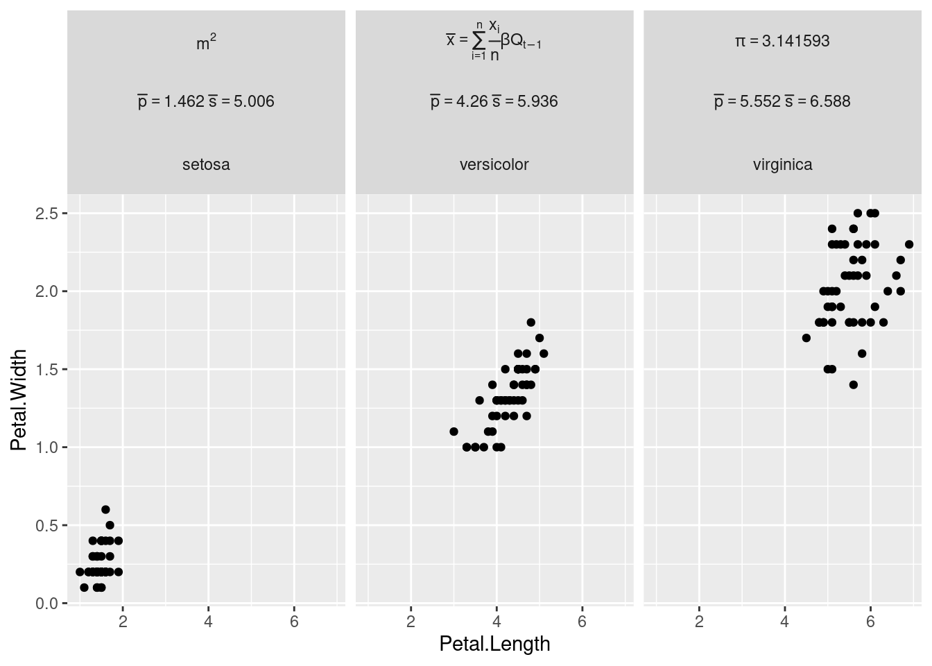

As shown in the example above, the labeller can parse:

A character vector such as “m^2” for simple formulas
An expression for more complex math with indices
The output of bquote to include numerical values in the formula. See also this answer on how to use bquote with numerical vectors of more than one value.
see this other answer on how to apply the labeller to one of the faceting variables only. In our case we apply it to the species_math variable only.

The syntax is different from Latex math formulas because label_parsed interprets labels as plotmath expressions. For example indices are written x_i in Latex and x[i] in plot math expressions, and Greek letters are written directly as alpha instead of \alpha in Latex. You can find many formulas in the help page of the plotmath function. Good luck with the plotmath examples.

Save plots to pdf

Use ggsave:

ggplot(mtcars, aes(mpg, wt)) + geom_point()
ggsave("mtcars.pdf")

Themes

Minimal theme

theme_minimal()

Geoms

Bar plots with geom_col

Use geom_col for bar plots where the height of the column represent the value of a variable. Use geom_bar for plots where the height of the column represents a count of number of occurrences.

geom_ribbon

Example from help(geom_ribbon):

 huron <- data.frame(year = 1875:1972, level = as.vector(LakeHuron))
 ggplot(huron, aes(year)) +
   geom_ribbon(aes(ymin = level - 1, ymax = level + 1), fill = "grey70") +
   geom_line(aes(y = level))

Add or remove lines at the border of the ribbon:

 ggplot(huron, aes(year)) +
   geom_ribbon(aes(ymin = level - 1, ymax = level + 1), 
               outline.type="lower", fill = "grey70", color="red") +
   geom_line(aes(y = level))

 ggplot(huron, aes(year)) +
   geom_ribbon(aes(ymin = level - 1, ymax = level + 1), 
               outline.type="lower", fill = "grey70", color="red",
               linetype=0) +
   geom_line(aes(y = level))

Palettes

Setting up colour palettes in R

To create a RColorBrewer palette, use the brewer.pal function. It takes two arguments: n, the number of colors in the palette; and name, the name of the palette. Let’s make a palette of 8 colors from the qualitative palette, “Set2”.

library(RColorBrewer)
brewer.pal(n = 8, name = "Set2") 
#[1] "#66C2A5" "#FC8D62" "#8DA0CB" "#E78AC3" "#A6D854" "#FFD92F" "#E5C494" "#B3B3B3" 
palette(brewer.pal(n = 8, name = "Set2"))

Use this palette in ggplot2

ggplot(iris, aes(x=Sepal.Length, y=Petal.Length, color=Species)) + 
    geom_point() +
    scale_color_brewer(palette = "Set2")

Manual colours

Use a named vector to set a palette in ggplot2 as explained in ggplot2 scale_manual

p <- ggplot(iris, aes(x=Sepal.Length, y=Petal.Length, color=Species)) +
        geom_point() 
p + scale_colour_manual(values = c(setosa='black', versicolor='red', virginica='green'))

Create a named palette using R colour brewer:

species_names <- c("setosa", "versicolor", "virginica") 
iris_palette <- setNames(brewer.pal(n=length(species_names), name='Set2'), 
                         species_names)
p + scale_colour_manual(values = iris_palette)

Display palettes

Display qualitative palettes:

display.brewer.all(type="qual")

Display all palettes

display.brewer.all()

Add more colours to a palette

Expand colour palettes in R

Expand from 8 colours to more colours:

mycolors <- colorRampPalette(brewer.pal(8, "Set2"))(nb.cols)

Text labels

ggplot2 text

Use position jitter

#  Reduce the number of points so it becomes more readable
iris2 <- iris %>% 
    group_by(Species, Petal.Width) %>%
    summarise(Sepal.Width = mean(Sepal.Width))
ggplot(iris2, aes(x = Petal.Width, y=Sepal.Width, color = Species)) +
    geom_text(aes(label = Species), 
              position=position_jitter(width=0.5,height=0.3),
              hjust="left") +
    # Expand the scale so that names are shown in full
    scale_x_continuous(expand = expansion(mult=c(0.1,0.5)))

Use repulsive textual annotations

ggplot(iris2, aes(x = Petal.Width, y=Sepal.Width, color = Species)) +
    ggrepel::geom_text_repel(aes(label = Species))

Change the text size

ggplot(iris2, aes(x = Petal.Width, y=Sepal.Width, color = Species)) +
    ggrepel::geom_text_repel(aes(label = Species), size=8)

More ggrepel examples

Justification

df <- data.frame(
  x = c(1, 1, 2, 2, 1.5),
  y = c(1, 2, 1, 2, 1.5),
  text = c("bottom-left", "bottom-right", "top-left", "top-right", "center")
)
ggplot(df, aes(x, y)) +
  geom_text(aes(label = text))
ggplot(df, aes(x, y)) +
  geom_text(aes(label = text), vjust = "inward", hjust = "inward")

Python compared to R

See also the python page for a comparison between pandas methods and R data frames functions.

l = c(1,2,3)
s = l
s[3]
[1] 3
s[3] = "a"
s
[1] "1" "2" "a"
l
[1] 1 2 3

Using the address function to see the address of these objects in memory We can see that s and l share the same address. The address only changes when we asign something to s.

library(pryr)
l = c(1,2,3)
s = l
address(l)
[1] "0x316f718"
address(s)
[1] "0x316f718"
s[3] = "a"
address(s)
[1] "0x36a7d30"
s
[1] "1" "2" "a"
l
[1] 1 2 3

Checking string objects

bla = "qsdfmlkj"
address(bla)
[1] "0x38e5120"
bli = bla
address(bli)
[1] "0x38e5120"
bli = paste(bli, "sdf")
address(bli)
[1] "0x38d1d60"

TODO Compare to the same code in python to see the difference between the above and passing by reference.

Shiny

K means example

App.R

Shiny tutorial lesson 1

“Note: Prior to version 0.10.2, Shiny did not support single-file apps and the ui object and server function needed to be contained in separate scripts called ui.R and server.R, respectively. This functionality is still supported in Shiny, however the tutorial and much of the supporting documentation focus on single-file apps.”

Tidyverse

dplyr

Group_by and summarise

library(dplyr)
cars %>%
    group_by(speed) %>%
    print(n=2) %>% # works because the print function returns its argument
    summarise(numberofcars = n(),
              min = min(dist),
              mean = mean(dist),
              max = max(dist))

## # A tibble: 50 × 2
## # Groups:   speed [19]
##   speed  dist
##   <dbl> <dbl>
## 1     4     2
## 2     4    10
## # ℹ 48 more rows

## # A tibble: 19 × 5
##    speed numberofcars   min  mean   max
##    <dbl>        <int> <dbl> <dbl> <dbl>
##  1     4            2     2   6      10
##  2     7            2     4  13      22
##  3     8            1    16  16      16
##  4     9            1    10  10      10
##  5    10            3    18  26      34
##  6    11            2    17  22.5    28
##  7    12            4    14  21.5    28
##  8    13            4    26  35      46
##  9    14            4    26  50.5    80
## 10    15            3    20  33.3    54
## 11    16            2    32  36      40
## 12    17            3    32  40.7    50
## 13    18            4    42  64.5    84
## 14    19            3    36  50      68
## 15    20            5    32  50.4    64
## 16    22            1    66  66      66
## 17    23            1    54  54      54
## 18    24            4    70  93.8   120
## 19    25            1    85  85      85

group_by() creates a tbl_df objects which is a wrapper around a data.frame to enable some functionalities. Note that print returns its output on a tbl_df object. So print() can be used inside the pipe without stopping the workflow.

Count and tally

Count the unique values of one or more variables

count(iris, Species, sort=TRUE)

is equivalent to

iris %>%
    group_by(Species) %>%
    tally(sort=TRUE)

The wt argument can be used to perform weighted counts

count(iris, Species, wt=Sepal.Length, sort=TRUE)

Across

Apply the same transformation to multiple columns, allowing to use select semantics inside summarise and mutate.

cars %>%
    group_by(speed) %>%
    summarise(across(dist, list(n = length , min = min, mean = mean, max = max)))

## # A tibble: 19 × 5
##    speed dist_n dist_min dist_mean dist_max
##    <dbl>  <int>    <dbl>     <dbl>    <dbl>
##  1     4      2        2       6         10
##  2     7      2        4      13         22
##  3     8      1       16      16         16
##  4     9      1       10      10         10
##  5    10      3       18      26         34
##  6    11      2       17      22.5       28
##  7    12      4       14      21.5       28
##  8    13      4       26      35         46
##  9    14      4       26      50.5       80
## 10    15      3       20      33.3       54
## 11    16      2       32      36         40
## 12    17      3       32      40.7       50
## 13    18      4       42      64.5       84
## 14    19      3       36      50         68
## 15    20      5       32      50.4       64
## 16    22      1       66      66         66
## 17    23      1       54      54         54
## 18    24      4       70      93.8      120
## 19    25      1       85      85         85

With trade data

summarise(across(all_of(c("tradevalue", "weight", "quantity")), sum, na.rm=TRUE))

Other examples from the help of the across function

# A purrr-style formula
iris %>%
    group_by(Species) %>%
    summarise(across(starts_with("Sepal"), ~mean(.x, na.rm = TRUE)))

## # A tibble: 3 × 3
##   Species    Sepal.Length Sepal.Width
##   <fct>             <dbl>       <dbl>
## 1 setosa             5.01        3.43
## 2 versicolor         5.94        2.77
## 3 virginica          6.59        2.97

# A named list of functions
iris %>%
    group_by(Species) %>%              # 
    summarise(across(starts_with("Sepal"), list(mean = mean, sd = sd)))

## # A tibble: 3 × 5
##   Species    Sepal.Length_mean Sepal.Length_sd Sepal.Width_mean Sepal.Width_sd
##   <fct>                  <dbl>           <dbl>            <dbl>          <dbl>
## 1 setosa                  5.01           0.352             3.43          0.379
## 2 versicolor              5.94           0.516             2.77          0.314
## 3 virginica               6.59           0.636             2.97          0.322

# Show all_of to select a vector of variables
iris %>%
    group_by(Species) %>%
    summarise(across(all_of(c("Sepal.Length", "Petal.Width")), 
                            ~mean(.x, na.rm = TRUE)))

## # A tibble: 3 × 3
##   Species    Sepal.Length Petal.Width
##   <fct>             <dbl>       <dbl>
## 1 setosa             5.01       0.246
## 2 versicolor         5.94       1.33 
## 3 virginica          6.59       2.03

More information in the vignette

vignette("colwise", package="dplyr")

The vignette mentions this about rename:

“across() doesn’t work with select() or rename() because they already use tidy select syntax; if you want to transform column names with a function, you can use rename_with().”

Mutate to create a new vector

Mutate multiple variables in the dataframe at once using the vars() helper function to scope the mutation: Note mutate_at has been superseded by the across function.

iris %>%
    mutate_at(vars(starts_with("Petal")), round) %>%
    head()

##   Sepal.Length Sepal.Width Petal.Length Petal.Width Species
## 1          5.1         3.5            1           0  setosa
## 2          4.9         3.0            1           0  setosa
## 3          4.7         3.2            1           0  setosa
## 4          4.6         3.1            2           0  setosa
## 5          5.0         3.6            1           0  setosa
## 6          5.4         3.9            2           0  setosa

Rename columns

rename_with from the dplyr package can use either a function or a formula to rename a selection of columns given as the .cols argument. For example passing the function name toupper or tolower:

library(dplyr)
rename_with(head(iris), toupper, starts_with("Petal"))
rename_with(head(iris), tolower, starts_with("Petal"))

Is equivalent to passing the formula ~ toupper(.x):

rename_with(head(iris), ~ toupper(.x), starts_with("Petal"))

To rename all columns, you can also use set_names from the rlang package. We now use paste0 as a renaming function. pasteO takes 2 arguments, as a result there are different ways to pass the second argument depending on whether we use a function or a formula.

rlang::set_names(head(iris), paste0, "_hi")
rlang::set_names(head(iris), ~ paste0(.x, "_hi"))

The same can be achieved with rename_with by passing the data frame as first argument .data, the function as second argument .fn, all columns as third argument .cols=everything() and the function parameters as the fourth argument .... Alternatively you can place the second, third and fourth arguments in a formula given as the second argument.

rename_with(head(iris), paste0, everything(), "_hi")
rename_with(head(iris), ~ paste0(.x, "_hi"))

rename_with only works with data frames. set_names is more generic and can also perform vector renaming

rlang::set_names(1:4, c("a", "b", "c", "d"))

Recode values in a vector

“Replace numeric values based on their position or their name, and character or factor values only by their name.”

char_vec <- sample(c("a", "b", "c"), 10, replace = TRUE)
recode(char_vec, a = "Apple")

Pipes

purrr

Hadley Wickham’s answer to a SO question Why use purrr::map instead of lapply?

Map a function to nested data sets

Load data

list.files(getwd())
forestEU_wide <- read.csv("Forest-R-EU.csv", stringsAsFactors = FALSE)
head(forestEU)

Pivot to long format

# at some pointin the future this will be called pivot_long
forestEU <- forestEU_wide  %>% 
      # select everything except the Year, then pivot all columns and put the value in area
      gather(-Year, key = "Country", value = "Area")

Tricks

David Robinson Ten tricks in the tidyverse

count with weight, sort and renamining count(x, …, wt = NULL, sort = FALSE, name = “n”)
creating variables in count()
add_count()
summarize with a list column (to create many models for example)
fct_reorder() + geom_col() + coord_flip()
fct_lump() to lump less frequent values together
use a log scale scale_x/y_log10
crossing()
separate()
extract() use a regular expression such as S(.*)E(.*) to extract series and episode from a string of the form “S32E44”.

Purrr

Interpolation

Interpolate for one country

country_interpolation <- function(df) {
    df <- data.frame(approx(df$Year, df$Area, method = "linear", n=71))
    df <- rename(df, Year = x, Area = y)
    return(df)
}
forestEU %>%
    filter(Country=="Austria") %>%
    country_interpolation()

Interpolate for all countries Perform the Interpolation on all countries

See documentation in * many models https://r4ds.had.co.nz/many-models.html * blog https://emoriebeck.github.io/R-tutorials/purrr/

forestEU_nested <- forestEU %>%
      # Remove empty area
      filter(!is.na(Area)) %>% 
      group_by(Country) %>%  
      nest() %>% 
      mutate(interpolated = map(data, country_interpolation))

# forestEU_nested %>% unnest(data)
# Unnest the interpolated data to look at it and plotting
forestEU_interpolated <- forestEU_nested %>% unnest(interpolated)

Read many csv

See iris_csv file created in the csv section of this document. Read these csv files into one data frame. Note the Species column has to be present in the csv files, otherwise we would loose that information.

iris_csv <- list.files(data_folder, full.names = TRUE) %>% 
    purrr::map_dfr(read_csv)

Write to many csv

#dir.create("output")
forestEU_nested <- forestEU_nested %>% 
    mutate(filename = paste0("output/", Country, ".csv"),
    wrote_stuff = map2(interpolated, filename, write.csv))

tidy evaluation

Advanced R metaprogramming section
Examples of tidy evaluation with plots

scatter_plot <- function(data, x, y) {
    x <- enquo(x)
    y <- enquo(y)
    ggplot(data) + geom_point(aes(!!x, !!y))
}
scatter_plot(mtcars, disp, drat)

Another example use of metaprogramming to change variables

add1000 <- function(dtf, var){
      varright <- enquo(var)
  varleft <- quo_name(enquo(var))
    dtf %>% 
            mutate(!!varleft := 1000 + (!!varright))
}
add1000(iris, Sepal.Length)

Tidy evaluation explained in French

Tidy select

Tidy select selection language explains the various selection function such as all_of, contains and starts_with.

library(dplyr)
iris2 <- head(iris, 1)
select(iris2, contains("w")) # Literal string
select(iris2, matches("w")) # Regular expression
select(iris2, starts_with("S"))
select(iris2, all_of(c("Sepal.Length", "Petal.Width")))

The selection can be inverted by using s minus sign in front of it. Not it’s not a question mark as explained in this SO answer because the selection fonctions return numerical vectors of integer column positions (not boolean values).

library(dplyr)
select(head(iris), -matches("w") )

tidyr

tidyr vignette on tidy data In the section on “Multiple types in one table”:

Datasets often involve values collected at multiple levels, on different types of observational units. During tidying, each type of observational unit should be stored in its own table. This is closely related to the idea of database normalisation, where each fact is expressed in only one place. It’s important because otherwise inconsistencies can arise.

Normalisation is useful for tidying and eliminating inconsistencies. However, there are few data analysis tools that work directly with relational data, so analysis usually also requires denormalisation or the merging the datasets back into one table.

Example use of tidyr::nest() to generate a group of plots: make ggplot2 purrr.

library(tidyr)
library(dplyr)
library(purrr)
library(ggplot2)
piris <- iris %>%  
    group_by(Species) %>% 
    nest() %>% 
    mutate(plot = map2(data, Species, 
                       ~ggplot(data = .x, 
                               aes(x = Petal.Length, y = Petal.Width)) + 
                           geom_point() + ggtitle(.y)))
piris$plot[1]
piris$plot[3]
piris$plot[2]

Time series

Moving averages

Use the rollmean function from the zoo package. It defaults to centered.

 library(zoo)
 x.Date <- as.Date(paste(2004, rep(1:4, 4:1), sample(1:28, 10), sep = "-"))
 x <- zoo(rnorm(12), x.Date)
 rollmean(x, 3, fill=NA)
 rollmean(x, 3, fill="extend")
 y <- x
 y["2004-01-15"] <- NA
 rollmean(y, 3, fill="extend") 
 # Returns NA values if there are not enough observations for the rollmean
 rollmean(y, 9, fill="extend") 
 rollmean(x, 9, fill="extend")

Working directory

Hadley Wickham on a Stackoverflow comment:

“You should never use setwd() in R code - it basically defeats the idea of using a working directory because you can no longer easily move your code between computers. – hadley Nov 20 ’10 at 23:44”

Content copied from my StackOverflow answer.

TLDR: The here package (available on CRAN) helps you build a path from a project’s root directory. R projects configured with here() can be shared with colleagues working on different laptops or servers and paths built relative to the project’s root directory will still work. The development version is at github.com/r-lib/here.

With git

You certainly store your R code in a directory. This directory is probably part of a git repository and/or an R studio project. I would recommend building all paths relative to that project’s root directory. For example let’s say that you have an R script that creates reusable plotting functions and that you have an R markdown notebook that loads that script and plots graphs in a nice (so nice) document. The project tree would look something like this

├── notebooks
│   ├── analysis.Rmd
├── R
│   ├── prepare_data.R
│   ├── prepare_figures.R

From the analysis.Rmd notebook, you would import plotting function with here() as such:

source(file.path(here::here("R"), "prepare_figures.R"))

Why?

From the Ode to the here package:

Do you: Have setwd() in your scripts? PLEASE STOP DOING THAT. This makes your script very fragile, hard-wired to exactly one time and place. As soon as you rename or move directories, it breaks. Or maybe you get a new computer? Or maybe someone else needs to run your code? […] Classic problem presentation: Awkwardness around building paths and/or setting working directory in projects with subdirectories. Especially if you use R Markdown and knitr, which trips up alot of people with its default behavior of “working directory = directory where this file lives”. […]

Install the here package:

install.packages("here")
library(here)
here()
here("construct","a","path")

Documentation of the here() function:

Starting with the current working directory during package load time, here will walk the directory hierarchy upwards until it finds a directory that satisfies at least one of the following conditions:

contains a file matching [.]Rproj$ with contents matching ^Version: in the first line

[… other options …]

contains a directory .git

Once established, the root directory doesn’t change during the active R session. here() then appends the arguments to the root directory.

The development version of the here package is available on github.

What about

What about files outside the project directory?

If you are loading or sourcing files outside the project directory, the recommended way is to use an environment variable at the Operating System level. Other users of your R code on different laptops or servers would need to set the same environment variable. The advantage is that it is portable.

data_path <- Sys.getenv("PROJECT_DATA")
df <- read.csv(file.path(data_path, "file_name.csv"))

Note: There is a long list of environmental variables which can affect an R session.

What about many projects sourcing each other?

It’s time to create an R package.

Further resources

Blogs

tinyverse “Lightweight is the right weight”
- Dirk Eddelbuettel dependencies
  
  “I relied on the liteq package by Gabor which does the job: enqueue jobs, and reliably dequeue them (also in a parallel fashion) and more. It looks light enough:”
```
  R> tools::package_dependencies(package="liteq", recursive=FALSE, db=AP)$liteq
  [1] "assertthat" "DBI"        "rappdirs"   "RSQLite"
```
  “Two dependencies because it uses an internal SQLite database, one for internal tooling and one for configuration.” All good then? Not so fast. The devil here is the very innocuous and versatile RSQLite package because when we look at fully recursive dependencies all hell breaks loose: Now we went from four to twenty-four, due to the twenty-two dependencies pulled in by RSQLite.”
Gavin Simpson My aversion to pipers shows an Hadley tweet explaining that pipe might not be good in package development.
5 R packages for text analysis https://towardsdatascience.com/r-packages-for-text-analysis-ad8d86684adb

Shiny apps by international organizations

The human mortality database short term mortality fluctuations visualization toolkit, Git repository, Plos One paper